Angelo Ricotta
Our natural world behaves mostly analogically,
at least at a macroscopic level, therefore to interface it to digital computers
one has to sample analog signals. The universally known sampling theorem,
credited to Nyquist and Shannon, but the story is more articulated [1] [9], states
that to reconstruct correctly the information carried by a bandlimited signal,
the sampling frequency ![]() must be at least twice
the highest frequency
must be at least twice
the highest frequency ![]() of the signal :
of the signal : ![]() . In practice we use
. In practice we use ![]() because there could be
ambiguity in reconstructing the component associated to
because there could be
ambiguity in reconstructing the component associated to ![]() and, depending on the
non ideal shape of real-world bandlimited spectra, also folding of the upper
part of the spectrum. In this form the theorem is always valid but sometimes it
is stated as
and, depending on the
non ideal shape of real-world bandlimited spectra, also folding of the upper
part of the spectrum. In this form the theorem is always valid but sometimes it
is stated as ![]() where
where ![]() is the bandwidth of
the signal. The last formulation implicitly assumes that the lowest frequency
is the bandwidth of
the signal. The last formulation implicitly assumes that the lowest frequency ![]() of the signal is zero,
of the signal is zero,
![]() , otherwise it is not generally true, as we will see. If the
sampling frequency
, otherwise it is not generally true, as we will see. If the
sampling frequency ![]() is lower than
is lower than ![]() , i.e.
, i.e. ![]() , each of the frequencies
, each of the frequencies ![]() above
above ![]() will be aliased, i.e. superimposed
or confused, in particular, with a
corresponding frequency
will be aliased, i.e. superimposed
or confused, in particular, with a
corresponding frequency ![]() in the range
in the range ![]() (page 1 of Fig.1) according
to the relation
(page 1 of Fig.1) according
to the relation ![]() or
or ![]() with
with ![]() integer (Fig.1).
integer (Fig.1).
Fig.1 Folding around the Nyquist frequency ![]() and its multiples [2].
and its multiples [2].
You may think of the diagram of Fig.1 as pages
of length ![]() that fold over each
other, in particular over the first, alternately like an “accordion-pleated”
[2] strip of paper. Because this phenomenon the spectrum of a signal, when
sampled, will be aliased or replicated over all the pages. When the spectrum of the signal is contained
entirely in one of the pages, the spectral aliases of the sampled signal will
not overlap. If the original spectrum is not on the first page, one of the
aliases will be positioned on the first page with the result of having
converted down the frequencies of the original spectrum without modification of
the bins power. The order of the bins of the original spectrum will be
preserved if the original spectrum of the signal is contained in the odd pages
and inverted for the even pages. All this occurs because sampling in time
domain is a multiplication of the signal by a comb of unitary pulses, which in
frequency domain becomes a convolution of the Fourier transformed unitary pulses
with the spectrum of the signal. A nice detailed explanation, both mathematical
and visual, is given in [4]. The complete spectrum of a sampled bandlimited
signal is constituted of replicas of the original spectrum symmetrically
disposed around multiples, positive and negative, of the sampling frequency, as
illustrated in Fig.2. For example, let the original spectrum (the diagram on
the upper side) be composed of two pure tones at 1 and 12 (arbitrary frequency units)
and of a continuous spectrum ranging from 6 to 7. Sampling the signal at 5 we
obtain the coloured diagram on the bottom, where we can see the symmetrical
replicas of the original spectrum centred at multiples of
that fold over each
other, in particular over the first, alternately like an “accordion-pleated”
[2] strip of paper. Because this phenomenon the spectrum of a signal, when
sampled, will be aliased or replicated over all the pages. When the spectrum of the signal is contained
entirely in one of the pages, the spectral aliases of the sampled signal will
not overlap. If the original spectrum is not on the first page, one of the
aliases will be positioned on the first page with the result of having
converted down the frequencies of the original spectrum without modification of
the bins power. The order of the bins of the original spectrum will be
preserved if the original spectrum of the signal is contained in the odd pages
and inverted for the even pages. All this occurs because sampling in time
domain is a multiplication of the signal by a comb of unitary pulses, which in
frequency domain becomes a convolution of the Fourier transformed unitary pulses
with the spectrum of the signal. A nice detailed explanation, both mathematical
and visual, is given in [4]. The complete spectrum of a sampled bandlimited
signal is constituted of replicas of the original spectrum symmetrically
disposed around multiples, positive and negative, of the sampling frequency, as
illustrated in Fig.2. For example, let the original spectrum (the diagram on
the upper side) be composed of two pure tones at 1 and 12 (arbitrary frequency units)
and of a continuous spectrum ranging from 6 to 7. Sampling the signal at 5 we
obtain the coloured diagram on the bottom, where we can see the symmetrical
replicas of the original spectrum centred at multiples of ![]() and also note that the
pure tones, originally positioned at 5 and 12, and then isolated, are now superimposed
to the borders of the continuous spectrum. Of course, when we sample a signal
with continuous spectrum for a finite duration
and also note that the
pure tones, originally positioned at 5 and 12, and then isolated, are now superimposed
to the borders of the continuous spectrum. Of course, when we sample a signal
with continuous spectrum for a finite duration ![]() , the spectrum of the sampled signal will be constituted of
discrete components (bins), whose frequency resolution is
, the spectrum of the sampled signal will be constituted of
discrete components (bins), whose frequency resolution is ![]() , which are not visible in Fig.2.
, which are not visible in Fig.2.
Fig.2 Replicas of the spectrum of a sampled
bandlimited or bandpass signal.
The “accordion-pleated” paper model leads to a
straightforward mathematical formulation.
Let ![]() be the bandwidth of the
signal to be sampled.
be the bandwidth of the
signal to be sampled.
The key conditions to
avoid the folding of the spectrum on itself, for ![]() integer,
integer,
![]() and
and ![]()
which means that the original spectrum of the
signal must be contained entirely in one of the pages of Fig.1. Actually the
spectrum could be segmented in different pages. In that case we have to state
the above conditions for each segment and others have to be verified so that the
segments will not fold on each other when the signal is sampled.
The connection between the page number ![]() and
and ![]() is
is ![]()
Isolating ![]() from the above inequalities
we have
from the above inequalities
we have
![]() (1)
(1)
and eliminating ![]() we obtain
we obtain ![]() from which
from which
![]() (2)
(2)
These are the fundamental formulae for undersampling (bandpass sampling, subsampling, downsampling, sub-Nyquist, super-Nyquist, harmonic sampling) even if I did not
use any of these terms in my original report [3] because, at
that time, I was not concerned about any specific terminology for this kind of
operation.
For example, let it be ![]() and
and ![]() . Applying (2)
we have
. Applying (2)
we have ![]() , i.e.
, i.e. ![]() , and then
from (1) we obtain all the allowable
sampling frequencies:
, and then
from (1) we obtain all the allowable
sampling frequencies: ![]() :
: ![]() ,
, ![]() :
: ![]() and, of course,
and, of course, ![]() :
: ![]() . As
anticipated, the order of the bins of the aliased spectrum of the bandpass
signal is reversed or not depending on the position of the original spectrum of
the signal to respect to the chosen
. As
anticipated, the order of the bins of the aliased spectrum of the bandpass
signal is reversed or not depending on the position of the original spectrum of
the signal to respect to the chosen ![]() : if the
corresponding
: if the
corresponding ![]() is odd the order is preserved, if it is even
the order is reversed.
is odd the order is preserved, if it is even
the order is reversed.
Note that for doing a correct
undersampling you cannot use all the sampling frequencies ![]() , in fact in the above example it would be
, in fact in the above example it would be ![]() which is clearly
wrong. If you are interested only in the lowest bound
which is clearly
wrong. If you are interested only in the lowest bound ![]() of the sampling
frequencies, substituting (2) into (1) the left term furnishes
of the sampling
frequencies, substituting (2) into (1) the left term furnishes
 (3)
(3)
which is the same as that reported in [4]. An
expression equivalent to (1), but in the time domain, is given in [5]. We did
not use the equal sign in (1) and (2) to avoid a possible folding and
ambiguities of the frequencies at the borders of the spectrum, but if the power
in the bins outside the open range ![]() is zero or negligible we may write
is zero or negligible we may write ![]() and
and  , i.e. we
have to consider the shape of the real-world bandpass spectrum and choose
, i.e. we
have to consider the shape of the real-world bandpass spectrum and choose ![]() so that to avoid ambiguities
and minimize the folding of the spectrum on itself. It is possible to give to
(3) a different form. Let it be
so that to avoid ambiguities
and minimize the folding of the spectrum on itself. It is possible to give to
(3) a different form. Let it be ![]() and call it “band
index”. Consider
and call it “band
index”. Consider  . The range of
 ![]() is
is ![]() , furthermore it is
, furthermore it is ![]() and then
and then ![]() . The
. The ![]() range is
range is ![]() and its diagram is shown
on Fig.3. Note that for
and its diagram is shown
on Fig.3. Note that for ![]() not
not ![]() .
.
Fig.3 Lowest bound of the sampling frequency normalized
to the bandwidth versus the band index.
In a recent article [6] were reported the two
formulae ![]() and
and ![]() to compute an allowable sampling frequency for
undersampling a bandpass signal, being
to compute an allowable sampling frequency for
undersampling a bandpass signal, being ![]() the carrier, and
the carrier, and ![]() the bandwidth of the
signal. The procedure to compute
the bandwidth of the
signal. The procedure to compute ![]() is: as a first
approximation put
is: as a first
approximation put ![]() , insert this value in
, insert this value in  then use this rounded-down integer value of
 ![]() to calculate the true
to calculate the true ![]() . I think that this method, as an illustration of the
undersampling concepts, is useless and even misleading at least for two
reasons: the first because it is not simpler than the more general approach given
by the inequalities (1) and (2), the second and worse, because it gives only a
single sampling frequency instead of all the permitted frequencies, and the
computed frequency is not even the lowest bound, but only that particular
sampling frequency for which the spectral aliases of the sampled signal are
centred on the pages of Fig.1. The above formulae express this last property in
a foggy way and even as an algorithm they are twisted, compared to the sunny
logic of (1) e (2). In fact take
. I think that this method, as an illustration of the
undersampling concepts, is useless and even misleading at least for two
reasons: the first because it is not simpler than the more general approach given
by the inequalities (1) and (2), the second and worse, because it gives only a
single sampling frequency instead of all the permitted frequencies, and the
computed frequency is not even the lowest bound, but only that particular
sampling frequency for which the spectral aliases of the sampled signal are
centred on the pages of Fig.1. The above formulae express this last property in
a foggy way and even as an algorithm they are twisted, compared to the sunny
logic of (1) e (2). In fact take ![]() and
and ![]() , being
, being ![]() and
and ![]() , as in the
preceding example, we will have
, as in the
preceding example, we will have ![]() , instead
the lowest bound for the sampling frequency is
, instead
the lowest bound for the sampling frequency is ![]() . If the only data at our disposal are
. If the only data at our disposal are ![]() and
and ![]() it is easy to switch
to the general method taking
it is easy to switch
to the general method taking ![]() and
and ![]() and carrying on the computation as I suggested.
Anyway, the formulae
and carrying on the computation as I suggested.
Anyway, the formulae ![]() and
and ![]() can be easily deduced from
can be easily deduced from ![]() . By
definition
. By
definition ![]() , therefore
, therefore ![]() is always satisfied, because implicitly
contained in (1): note that you cannot use every
is always satisfied, because implicitly
contained in (1): note that you cannot use every ![]() for undersampling, as already shown, because
you have to satisfy the other constraint. To deduce
for undersampling, as already shown, because
you have to satisfy the other constraint. To deduce ![]() , assume
, assume ![]() , i.e. the arithmetic mean of the two bounds of (1). Doing
the following sequential manipulations we have:
, i.e. the arithmetic mean of the two bounds of (1). Doing
the following sequential manipulations we have:  .
.
Because ![]() , and substituting
, and substituting
![]() deduced from (1), we finally obtain
deduced from (1), we finally obtain  . The substitution
 ![]() produces, as expected, an
produces, as expected, an ![]() lower than the arithmetic mean assumed in
advance. Eventually it is
lower than the arithmetic mean assumed in
advance. Eventually it is ![]() and then
and then ![]() with
with ![]() . A more perspicuous deduction can be done from the key
conditions [3] considering that the aim of the
above formulae for
. A more perspicuous deduction can be done from the key
conditions [3] considering that the aim of the
above formulae for ![]() is to centre the spectral aliases of the sampled
signal on the pages of Fig.1. It has to be
is to centre the spectral aliases of the sampled
signal on the pages of Fig.1. It has to be ![]() from which
from which ![]() .
.
Even in practical applications it is important
to be able to calculate all the permitted sampling frequencies, because you may
have some constraints that force you to choose a particular range of sampling
frequencies, so that it is better to rely on the general method for this
computation.
My interest in signal processing started in the
mid of 1975 when I began doing my thesis in Physics [7] which consisted in the
design and in the realization of a SODAR system for use in atmospheric boundary
layer studies. For the hardware I basically followed the work done by E.J.Owens
[8], adding some original solutions, anyway I was the first in Italy to design
and build a SODAR system that really worked, and even today many people use my scientific
and technical ideas and solutions,
some of which are described in [3] [7] [10], even if not all of them recognize it. SODAR is
the acronym of SOund Detecting And Ranging and it is an acoustic RADAR which
emits in the atmosphere short acoustic bursts which are scattered by
turbulence. The repetition rate of the bursts is, normally, between 3 and 6
seconds depending on the spatial range to be explored. The emitter is usually a
power loudspeaker, placed at the focus of a microwave parabolic dish generally
enclosed in an acoustic shield to attenuate the environmental noise. There are
also SODARs whose antennas are constituted of an array of loudspeakers. To
respect to the frequency range emitted there are, basically, two kind of instruments: low and high frequency SODARs. Typically,
the low frequency range is 1000-3000 Hz, the high frequency 5000-7000 Hz. In
Fig.4 and Fig.5 are shown the antennas of recent versions of SODARs I contributed
to design: the big truncated cone-shaped antennas of Fig. 4 are for
low-frequency range, the three horn-reflectors of Fig.5 are for high-frequency
range.
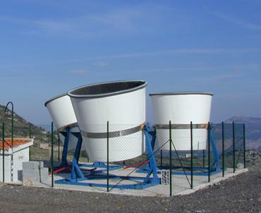
Fig.4 Antennas of the low-frequency SODAR system
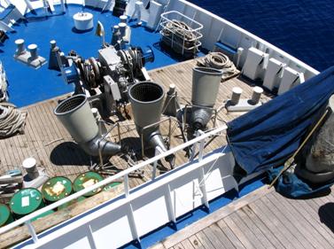
Fig.5 Antennas of the high-frequency SODAR system
During the 1976, and for many years after, the
first version of the SODAR, and its upgrades, I designed and built personally,
were extensively used in measurement campaigns and there emerged the need of an
efficient sampling of the signal and the necessity of a real-time processing of
the data. The first need came also from the fact that we had old computers with
limited A/D and poor storage units, the second because we needed the wind
profiles immediately for certain applications in the air pollution monitoring. The
SODAR is capable of producing a cumbersome amount of data even for today
standards, especially if you want to store the raw data for advanced future
analysis and because you have to digitize the signal continuously for many
days, and sometimes for months. So that I had to reduce the rate and the amount
of sampled data without losing the information we were interested on. The
solution proceeded by successive approximations. My first approach was hardware
and I realized, in 1980, an audio heterodyne that
translated down the spectrum of the echo. It was also tried the decimation of the
sampled data, comparing the spectra before and after and observing empirically that,
in certain conditions, the result was only a down translation of the frequency
bins without modification of the bins power. Then at the beginning of 1981 I
ran into [2], p.230, and imagined that the “accordion-pleated” paper model had
a useful mathematical formulation in terms of the fundamental formulae (1) and
(2) for undersampling shown above. Only much more later I read [4] and [5] and
realized that, at least (1) was already known, even if the topic was understated
and treated differently (it was never named undersampling but “bandpass sampling
theorem”) and partially and without proof in the quoted references, instead I
think that my proof is simple and smart. In [4] the fundamental formula is
stated differently and in the time domain instead of frequency domain, as I
did. Furthermore no formula for ![]() is given. In [5] the “bandpass
sampling theorem” is listed among the problems left to the reader and the
formula shown refers only to the critical sampling frequency (3), but one of
the terms may suggest, to an attentive reader, the way to compute
is given. In [5] the “bandpass
sampling theorem” is listed among the problems left to the reader and the
formula shown refers only to the critical sampling frequency (3), but one of
the terms may suggest, to an attentive reader, the way to compute ![]() . At that time, to my knowledge, people working on SODAR
systems did not use the undersampling technique to digitize the signal, and
even FFT was not so popular. Hence I think I was the
first to introduce the undersampling in this area, and in a very simple
form well suited for practical use. My fault was not to publicize enough my
results with the consequence that
a few people have tried to catch the merit for them even people I
informed of personally. But, even if my report of 1983 was late, having I
achieved the results in 1981 and even before, the papers of the others are all
of two and more years later and, in a number of cases, I know why: at the
beginning they did not believe in my results!
. At that time, to my knowledge, people working on SODAR
systems did not use the undersampling technique to digitize the signal, and
even FFT was not so popular. Hence I think I was the
first to introduce the undersampling in this area, and in a very simple
form well suited for practical use. My fault was not to publicize enough my
results with the consequence that
a few people have tried to catch the merit for them even people I
informed of personally. But, even if my report of 1983 was late, having I
achieved the results in 1981 and even before, the papers of the others are all
of two and more years later and, in a number of cases, I know why: at the
beginning they did not believe in my results!
The emitted signal of the SODAR is a sinusoidal
burst typically of 100 milliseconds every 6 seconds. The receiver channels open
after the emission of the bursts. Basically, the signal received is strongly
modulated in amplitude at a low frequency, broaded in frequency by turbulence
and shifted in frequency because the Doppler effect, furthermore it is embedded
in a variable amount of environmental noise. With the SODAR it is possible to
visualize the atmospheric turbulence and measure the wind profile remotely up
to ![]() to the first zeros,
where
to the first zeros,
where ![]() is the duration of the
burst. In our case
is the duration of the
burst. In our case ![]() and then
and then ![]() centred on
centred on ![]() , the transmitted frequency. The received signal has a spectrum
that looks like that of Fig.6, for a given segment of data.
, the transmitted frequency. The received signal has a spectrum
that looks like that of Fig.6, for a given segment of data.
Fig.6 Received power spectrum with very good
S/N ratio
Our aim is to measure the vertical profiles of
the speed and direction of the wind and the intensity of turbulence for each
scan or for a number of averaged scans and at a number of height levels. Before
digitizing we have to filter the signal with a bandpass filter with bandwidth ![]() , as shown in Fig.6, to avoid aliasing too much out of band
noise. Furthermore, I lock the sampling frequency
to the transmitted frequency to compensate for possible relative drifts that
influence directly the precision of the wind measurement. Moreover, when the
frequency bands of the three antennas are separated in such a manner to not
interfere each other and to satisfy, in the whole, the requirements for
undersampling, the three received signals are mixed together [10] before
sampling, reducing at one third the required sampling rate. In a particular
arrangement the whole bandwidth of the low frequency SODAR was
, as shown in Fig.6, to avoid aliasing too much out of band
noise. Furthermore, I lock the sampling frequency
to the transmitted frequency to compensate for possible relative drifts that
influence directly the precision of the wind measurement. Moreover, when the
frequency bands of the three antennas are separated in such a manner to not
interfere each other and to satisfy, in the whole, the requirements for
undersampling, the three received signals are mixed together [10] before
sampling, reducing at one third the required sampling rate. In a particular
arrangement the whole bandwidth of the low frequency SODAR was ![]() so that the numbers
are the same as in the previous example, except for the measuring units, which
are uninfluential in this context. This is the moment when undersampling enters
the scene: the ratio
so that the numbers
are the same as in the previous example, except for the measuring units, which
are uninfluential in this context. This is the moment when undersampling enters
the scene: the ratio ![]() determines, in the
example shown, the maximum factor of reduction on the number of sampled data
which is a great saving in memory storage and a strong reduction (considering
also the reduction in the sampling rate by mixing, when possible, of the three
received signals) of the sampling rate that speed up the data analysis, permitting
the real-time processing with cheaper instrumentation. After having undersampled
the signal of each scan, we partition them in a number of segments and for each
segment we apply the FFT to extract the spectrum shown in Fig.6.
determines, in the
example shown, the maximum factor of reduction on the number of sampled data
which is a great saving in memory storage and a strong reduction (considering
also the reduction in the sampling rate by mixing, when possible, of the three
received signals) of the sampling rate that speed up the data analysis, permitting
the real-time processing with cheaper instrumentation. After having undersampled
the signal of each scan, we partition them in a number of segments and for each
segment we apply the FFT to extract the spectrum shown in Fig.6.
In the backscattering mode, i.e. receiver
coaxial or coincident with the transmitter, the axial component of the wind is
given by
![]() (4)
(4)
where ![]() is the sound velocity,
is the sound velocity,
![]() the transmitted
frequency and
the transmitted
frequency and ![]() the received
frequency. This is a first order approximation but it is pretty good in our
atmosphere because
the received
frequency. This is a first order approximation but it is pretty good in our
atmosphere because ![]() . Typically the received frequency is defined as the first
normalized moment of the spectrum
. Typically the received frequency is defined as the first
normalized moment of the spectrum
in which ![]() is the
interval shown in Fig.6,
is the
interval shown in Fig.6, ![]() is the power of the
is the power of the ![]() bin and
bin and ![]() is the resolution of the spectrum. In a typical triaxial
arrangement the antennas are positioned as in Fig.7
is the resolution of the spectrum. In a typical triaxial
arrangement the antennas are positioned as in Fig.7
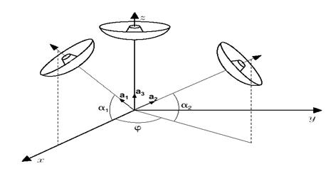
Fig.7 Orientation of the antennas of a triaxial
SODAR system
Having computed the three axial components ![]() ,
, ![]() , of the wind
, of the wind ![]() with the formula (4),
we need, for meteorological use, to transform them in cartesian components
with the formula (4),
we need, for meteorological use, to transform them in cartesian components ![]() ,
, ![]() , directed respectively along the axes
, directed respectively along the axes ![]() of a orthogonal frame
of reference. By definition is
of a orthogonal frame
of reference. By definition is ![]() and
and ![]() where
where ![]() and
and ![]() are
respectively the unit vectors of the antennas axes and of the cartesian axes. It
is
are
respectively the unit vectors of the antennas axes and of the cartesian axes. It
is
![]() (5)
(5)
in which we use the summation convention for
the repeated indices in the products. It is ![]() hence
hence ![]() with
with ![]() . Because we
already know
. Because we
already know ![]() from (4), knowing also
the geometric coefficients
from (4), knowing also
the geometric coefficients ![]() (cosine directors) we will be able to solve (5) to respect to the
three unknowns
(cosine directors) we will be able to solve (5) to respect to the
three unknowns ![]() . For the particular orientations depicted in Fig.7, we have
. For the particular orientations depicted in Fig.7, we have
![]()
hence

Solving to respect to
the ![]() we finally obtain
we finally obtain

Eventually, what began with undersampling SODAR
signals, has given its fruits. We are able to save, plot, print wind and
intensity profiles of the atmospheric boundary layer, up to about
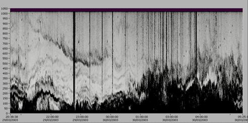
Fig.8 Vertical profile of the intensity of the
vertical backscattered signal versus time.
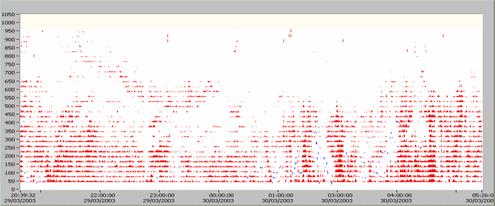
Fig.9 Vertical profile of the vertical wind
component versus time.
REFERENCES
[1] Abdul J. Jerry, “The Shannon Sampling
Theorem – Its Various Extensions and Applications: A Tutorial
Review”, Proc. of IEEE, vol.65, no. 11,
November 1977.
[2] Julius S. Bendat, Allan G. Piersol,
“Random Data: Analysis and Measurement Procedures”, Wiley-Interscience, 1971,
(p.230).
[4] E.
Oran Brigham, “The Fast Fourier Transform”, Prentice-Hall, Inc., 1974, (p.87).
[5] “Reference
Data For Radio Engineers, Fifth Edition”, Howard W. Sams & Co., Inc., ITT,
1970, (p.21-14).
[6] Bonnie
Baker, “Turning Nyquist upside down by undersampling”, EDN 12 May 2005.
[7] Angelo Ricotta, “Development of an
acoustic radar and its applications to the planetary boundary layer dynamics
studies”, Thesis in Physics,
[8] E. J. Owens, NOAA MARK VII Acoustic Echo
Sounder, NOAA Tech. Mem.,
[9] P. L. Butzer, J. R. Higgins, R. L. Stens,
“Sampling theory of signal analysis”, Development of Mathematics 1950-2000,
Editor J. P. Pier, Birkhäuser, 2000.
[10] A. Ricotta, M. Berico, “Triaxial Sodar”, Technical Report LPS 80-6, LPS-CNR, Frascati, 1980.